


Chaos theory in Einstein’s gravity may hold clues to the early universe
The only proven chaotic solution to general relativity just might be a clue to understanding time and quantum gravity

The only proven chaotic solution to general relativity just might be a clue to understanding time and quantum gravity
My first exposure to chaos theory was through the character of Prof. Malcolm in the novel Jurassic Park. Author Michael Crichton portrayed chaos theory as the underlying mathematical structure that led to the Robert Burns phrase, in Scottish dialect, “the best laid schemes o’ mice an’ men. Gang aft a-gley”.
The events of Jurassic Park were certainly a-gley, but you don’t need chaos theory to explain them, just Murphy’s law. Bad outcomes are the product of being over-confident and over-optimistic and assuming everything will go your way.
Chaos theory itself just didn’t play a role.

Chaos theory is responsible for the “butterfly effect”. A butterfly flaps its wings in China and it rains in New York City because the flapping of the wing causes a cascade of energy from smaller to larger scales, exactly the opposite of how things are “supposed” to work.
You don’t need to watch butterflies in China and correlate them with weather statistics in New York City, though, to understand chaos. All you need is a pendulum.
Chaotic systems have something called “sensitive dependence on initial conditions”. That means that not only can a butterfly in China cause rain in New York, but if you tried to repeat that experiment you would never succeed. You can never replicate the exact conditions. For scientists, it was a nail in the coffin of being able to predict the future with any precision, even without quantum mechanics to throw a wrench into everything.
Let’s look at an example. Take a pendulum. It has two numbers to describe its state at any time: position, given by its location along its swing, and momentum, which is just the product of its mass and its velocity. If you plot those two numbers on a grid, position on the horizontal axis and momentum on the vertical, for a series of times, you will see that the pendulum traces out a line. The grid is called the pendulum’s phase space. The line is its phase space trajectory.
You can learn all about phases spaces in my article:
A Visual Introduction to Classical Mechanics in Phase Space
An exploration of oscillators from springs to chaos.medium.com
Suppose you start a chaotic pendulum from a position and momentum (x,p). You record its trajectory on your grid. Now, start it at a very slightly different spot, (x+δ, p+ε). The new trajectory will diverge from the old one. For a non-chaotic pendulum, however, it will either converge or stay very close. This is what sensitive dependence on initial conditions means.
That divergence isn’t exponential in many cases, however, because chaotic systems have what are called strange attractors, which is where a set of initial conditions, called a basin of attraction, is attracted to a particular region of the phase space. That means that a chaotic pendulum, when started in a basin of attraction will tend towards a similar trajectory as from other points in the basin, but never the same trajectory, nor even crossing another one.
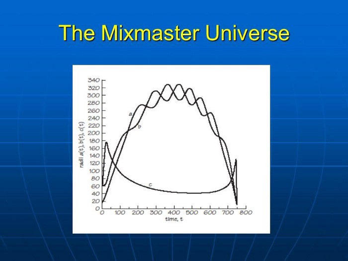
Chaotic systems have strong mixing properties. The Mixmaster universe — an early universe cosmology discovered by Charles Misner in the 1960s — is named, not after somebody named Mixmaster, not after a “Mixmaster” equation, but after popular mixer.

Not that mixer.
This one:

The Sunbeam Mixmaster, helping lonely housewives bake cakes from rationed supplies all through World War II.

The Mixmaster universe is homogeneous, meaning that, like most cosmological models, it assumes that the density of matter is the same throughout the universe. There are no irregularities. Everything is smoothed out.
It is not, however, an isotropic universe. Rather, it is anisotropic meaning that the universe may behave differently in different directions. You can think of a sphere as being an isotropic solid whereas an ellipsoid or oblate sphere is anisotropic.
We know from our best observations that our universe is homogeneous and isotropic. Therefore, the Mixmaster universe, if it existed, had to have been a feature of the very early universe. The universe would have started anisotropic and quickly converged to an isotropic form.
The Mixmaster is also a chaotic universe unlike the nice smoothly expanding one we live in today.
It expands and contracts repeatedly in one direction while expanding in the other, then those directions switch places. Hence it would have behaved like a three dimensional mixer, squeezing and blowing up repeatedly and randomly.
Misner thought the Mixmaster universe could explain why the Cosmic Microwave Background (CMB) was so well mixed. This could not have happened through ordinary electromagnetic or other forces because the parts that appear well mixed were too far apart for light to have traveled between them. It could only have happened gravitationally, based on the way the universe expanded.
Astrophysicists now believe that inflation caused the mixing, not by mixing at all but by stretching all the irregularities out like hand tossed pizza dough. Inflation fits the data better. Nevertheless, the mixmaster universe is the only solution to Einstein’s equations that has been proved to be chaotic. We have suspicions about other ones.
While chaos is an easy enough concept to understand, it is notoriously difficult to prove. Most of the chaotic systems we know about are one or two dimensional and the standard way to prove chaos in a multi-dimensional system is actually to reduce it to a one dimensional problem. Thus, proving a theory of a four dimensional cosmology to be chaotic was a huge achievement which went on unresolved for 30 years after it was proposed because of issues that are unique to relativity.
But first, what does chaos have to do with mixing?
In the 19th century, scientists were trying to understand the mathematics of how substances mixed, under what conditions could they be considered to be mixed, and what processes caused mixing.
They found four levels of mixing: ergodic, weakly mixed, strongly mixed, and Bernoulli shifted.
Suppose you are making a rum and coke and you have 10% rum and 90% coke. You can make one of four versions depending on how you mix it.
An ergodic cocktail is the least well mixed and means that if you take any volume of the rum and coke it will be 10% rum on average over time. That means that the proportion of rum at any specific time could be anything.
For a weakly mixed cocktail, the volume has 10% rum except once in a while.
For a strongly mixed cocktail, the proportion of rum is always 10%.
A Bernoulli shift cocktail is not only always 10% rum, but the configuration of the cocktail is completely random at every moment, so it isn’t just the proportion that is exact, it is never the same from moment to moment. You can think of this as a cocktail that is not only well mixed but in a constant state of agitation.
Bernoulli shift mixing is also called phi-mixing (as in the Greek letter phi) and is a special kind of mixing because it is pseudo-random. It can be used for pseudo-random number generators and may be responsible for Brownian motion. Many chaotic systems exhibit this kind of mixing including the Mixmaster universe.
If the rum and coke isn’t even ergodic, by the way, then you can’t say it is mixed at all. Have fun drinking that.
It’s time to look at some examples of chaotic systems.
The easiest way to understand a chaotic system is to use what are called maps which are simply relationships between the system state x at a time n and a time n+1. If it is a one dimensional system, then x is just a number.
The logistic map is one of the oldest chaotic maps and models the growth and collapse of populations. The logistic map isn’t always chaotic. Rather it may or may not be depending on the size of a controllable parameter.
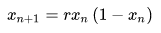

The controllable parameter here is r and the only other thing you can control is where it starts. If you let this map run for a while (easy enough with a little python code), it will tend to either converge to one or two or more points or it will be completely random. You can collect all these convergence points into a diagram called a bifurcation diagram. I have created one by running the map for 1000 iterations for 10000 values of r and plotting the final 100 iterations for each r (see below).
You can tell by looking at the diagram where it becomes chaotic because it looks messy. Those 100 values are all over the map. But a mathematical way of seeing it is by calculating the Lyapunov exponent which is a measure of how fast two neighboring trajectories in its phase space diverge. If this exponent is negative or zero it means that the system converges to a particular state called a fixed point or becomes periodic, and it is not chaotic. If it is positive, it is chaotic.
One of the nifty features here is you see that the state goes through something called “period doubling” as it heads towards chaos. It starts out for small r, less than about 3, converging to a single fixed point. After that, it ping pongs between two states. Then it doubles again to four. Each time it doubles, the Lyapunov exponent hits zero, kissing chaos, and then drops down again before going up. You can’t really see it but the periods continue to double, 2, 4, 8, 16, 32, but the range over r that they spend at each one get shorter. You can then see that after r=3.57 or so it becomes chaotic.
There are still short periods where it goes back to being non-chaotic. You can see those as white bars in between the randomness. I have tried to show this explicitly by coloring the chaotic Lyapunov exponents in red and the non-chaotic in black.

Another example are Chebyshev polynomials. There are an infinite number of these and they are all powerfully chaotic.
Here is a third order Chebyshev:

These maps are so chaotic they can stand in for completely random noise.

Chebyshev polynomials are also used in cryptography because they are so unpredictable but very symmetrical about 0.
Now, let’s talk about chaos in the Mixmaster universe.
The Mixmaster introduces three scale factors, a, b, and c, one for each spatial direction. Because they are homogeneous, these change with time but not with space. On the other hand, because they can all be different values, the universe is not isotropic.
You can compare the Mixmaster universe below to the standard cosmology, the FLRW universe, which only has the one scale factor for all three directions.

In order to prove that the Mixmaster universe is chaotic, you have to reduce it to a one dimensional map.
The Einstein equations guarantee that one of the scale factors, say c, depends on the other two, a and b, so it is already only two dimensions.
Now, two dimensions is still too many in this case and we can reduce it further to one using a mathematical trick called a Poincaré return mapping, section, recurrence map, or map. The map simply says that if you have some two dimensional or more space then your trajectories in that space must pass through a cross section of it.
If the return mapping is chaotic then the higher dimensional one must be. We can show that that mapping is chaotic for the Mixmaster.

Unfortunately, that isn’t enough in Einstein’s universe because we can always choose new coordinate systems and how can we know that there isn’t a coordinate system that just eliminates the chaos completely? Lyapunov exponents, in particular, are coordinate dependent and so unreliable as an indicator of chaos in this case.
A coordinate independent fractal method was devised in the late 90’s, 30 years after Misner introduced the universe, and showed that the Mixmaster universe is truly chaotic.
This fractal method, rather than looking at sensitive dependence on initial conditions, showed that the dynamics of the Mixmaster universe contain a strange repeller which is similar to a strange attractor but repulsive, in that the system tends to flow strangely away from it rather than strangely towards it. This is sort of like the top of a hill rather than a valley.
The set of initial conditions that tends to be attracted to a particular attractor or repelled by a repeller is called its basin of attraction or repulsion. If that basin has a boundary (border) that is fractal, then you know that it is a strange attractor or repeller, and the system is chaotic.
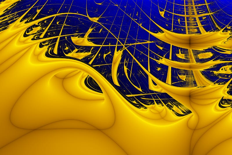
For example, the two dimensional system:

has a fractal basin boundary which you can see in all the peaks:

The Mixmaster universe has a similar fractal boundary to its repeller. At this point, the question was finally settled.
Unfortunately for the mathematics, all interest in the Mixmaster universe disappeared as inflationary theory took hold as a superior explanation of the CMB.
Still I think that the Mixmaster universe is worth studying for a few reasons.
The main reason is because we expect that there is a lot more chaos buried in general relativity, but the equations of relativity (there are ten of them) are so complex that we have to make simplifications like this. The Mixmaster is a guide towards finding those regions of chaos.
Another reason is that the Mixmaster universe scenario might show up on quantum scales where fluctuations can generate all kinds of extreme geometries. In that case, the Mixmaster might represent chaotic bubbles in the quantum foam at the Planck length. This might have all kinds of consequences for understanding the relationship between gravity and vacuum fluctuations, which may help explaining Dark Energy. In particular, studies of quantum versions of the theory applied to the early universe are on-going.
Another reason why the Mixmaster might be important is because chaos may be critical to explaining the thermodynamics of gravity, including black hole thermodynamics, as well as randomness in general relativity. Randomness within gravity itself is one candidate for explaining the arrow of time because it generates a direction of flow in a universe where time would otherwise be like any other direction. That flow may be how we experience time moving.
One thing is certain, the Mixmaster will always be a clear indicator that chaos lives within the beating heart of the universe.
Misner, Charles W. “Mixmaster universe.” Physical Review Letters 22.20 (1969): 1071.
Barrow, John D. “Chaotic behaviour in general relativity.” Physics Reports 85.1 (1982): 1–49.
Bergeron, Hervé, et al. “Quantum Mixmaster as a model of the Primordial Universe.” Universe 6.1 (2020): 7.