


A Visual Introduction to Classical Mechanics in Phase Space
An exploration of oscillators from springs to chaos.

Classical mechanics is one of the crowning achievements of the 17th through 19th centuries. Using only a few concepts like action and energy, we can determine the trajectories of countless particles and fields, even living things.
Many of us are familiar with mechanics. There is the classic parabolic trajectory of a ball thrown at a velocity both vertical and horizontal under gravity. The kinetic energy of the throw become potential energy as the ball rises and slows, then converts back into kinetic energy as it returns to Earth.
To understand the motion of the ball, we need to predict two quantities: position and momentum (which for constant mass is just mass times velocity). And indeed, in all of classical mechanics and even quantum mechanics, position and momentum show up. Sometimes these quantities are not exactly position and momentum, they are just “coordinates” and “conjugate momenta”. Yet, even when studying a gas of trillions and trillions of particles, the mechanics can be described as position and momentum of each one.
Understanding how these systems behave is important to many fields including rocket science, electrical and mechanical engineering, biology, and chemistry.
Phase Spaces with Visual Examples
A space is some region where all values with certain properties exist.
The space of all possible positions and momenta of your system, whether it is the position and momentum of a ball thrown up in the air, the oscillations of a spring, or a trillion particles, is called its phase space.
So, for example, in a one dimensional system like a ball thrown directly upward or a spring, the phase space is two dimensional: position and momentum. For a trillion particles in a three dimensional box, the phase space has six trillion dimensions, three position and three momentum for each particle. When we describe the position and momenta of every particle at one moment in time, it is called the state (sometimes microstate if we are talking about statistics). Every state of the system can be represented as a point in the phase space.
As an example, let’s take a spring with a mass on the end like this.

A spring is an example of an oscillator, something that has a repetitive or periodic motion. Here is an animation of how the spring oscillator appears versus what it looks like in phase space:
The above example is just one possible trajectory for the spring. I can change the size of the oval by changing the input velocity of the spring.
Springs like this have circular motion in phase space because they are neither forced nor damped, nor do they have any nonlinear behavior. Here are five different trajectories in phase space. Each one has a different initial condition (position and velocity).

Each color is a different trajectory over time with a different initial position and velocity. What this says is that any spring system in phase space looks like an oval shape. Those with less initial velocity have smaller ovals. Those with more have larger ovals.
This kind of spring isn’t that realistic because it goes on bouncing forever and ever like a perpetual motion machine. We should put some damping on it.
Damping can come from internal friction and heat loss of the spring. A damped spring system looks like this:

Now, instead of making big ovals, the phase space becomes a spiral because the position and momentum are “spiraling” into the 0 position and 0 momentum state which is the spring’s rest, neutral, or ground state.
Here are five random trajectories with random initial positions and velocities:

See how easy it is to visualize many, many solutions of the same equations in phase space? It also tells us a lot about what kind of system this is.
The damped spring system is not periodic now. Instead it goes to a “fixed point”. The system always heads straight to the point (0,0) and then it never leaves. This is a “stable” fixed point because if I disturb the oscillator in that state it will come back to it.
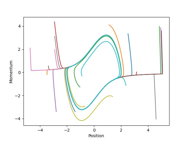
Let’s try one more 1-D oscillator. This time something called the Van der Pol Oscillator which is a nonlinear oscillator common in electrical circuits and vacuum tubes.

With this one, we can see an oscillator that has a limit cycle attractor. This is a kind of feature we don’t find in simple spring systems. If we were to drive a spring mass system with a Van der Pol oscillator, we might see something like this:

Here is the same oscillator’s phase space with 20 different initial conditions, one for each color. Each one is drawn to the limit cycle.
Chaotic systems, on the other hand, don’t have periodic attractors. They have “strange” attractors where they sort of follow an attractor, but they never hit the same state twice. Because they avoid hitting a state twice, they are never periodic. They always hit new states. Here’s an example in a three dimensional phase space:
The ball rolls around loops that appear to follow a pattern, but that pattern is never quite repeated. (Discounting the repetition of the animation.) Here is what that looks like in time in the x variable:

That is what chaos looks like. It never repeats and never hits the same point in phase space twice. Yet, it is deterministic not random. Every point in phase space is precisely determined by the equations and the initial conditions.
Higher Dimensions and Curved Geometries
In higher dimensions, dynamical systems become harder to visualize in phase space but the concepts are no less important. Indeed, phase spaces can have infinite dimensions in which case they become functional spaces like Hilbert spaces (common in signal processing and quantum field theory). Many of the concepts such as attractors, fixed points, and periodicity carry over, although limit cycles are less common outside of two dimensional phase spaces.
Beyond flat planar geometries, we can also carry these concepts into what are called symplectic geometries, which are, roughly speaking, non-Euclidean geometries that have the ability to be phase spaces. So, for example, these could be curved spaces embedded in a flat space of a higher dimension such as with orbits, or they could be in curved spaces like the surface of planets or even curved spacetime as in relativity. Most dynamical systems can be described as existing in symplectic geometries, provided they have even dimension phase spaces (which is generally true).
Conclusion
What I have shown you here is only a small slice of classical mechanics with phase spaces. The take away here is that phase space analysis is a powerful way to study dynamical systems and that we can understand a lot about a system just from its phase space behavior. It also leads to understanding aspects of dynamics like complexity and chaos, even what distinguishes living things from non-living dynamical systems. Indeed, you would expect the dynamics of a living thing, even a bacterium, to look very different from either a periodic or chaotic system. Instead it will be complex, non periodic, but also structured. If the question “what is life?” has an answer it will be a description of its phase space.